
It's been a while since I published my previous article from this series, so I decided that it is a perfect time to catch up. Today we are going to talk about one of the oldest and most commonly used types of databases - relational ones. Relational databases have been around since the late 60s - early 70s, long time before I was born, and they remain the most commonly used type of databases even today. It is hard to find a developer who has never worked with SQL or relational DBs, but not many understand how they work under the hood, therefore, our goal today is to fix that.
Before we start, I highly recommend you to check the first two articles from this series, namely How in-memory DB indexes work and How NoSQL DBs work and when to use them, if you haven't had a chance to read them yet.
B-Tree Index
As you probably know, it is always good to have a primary key in your relational DB table to uniquely identify one and only one row, which makes it easier to maintain the data and potentially increase read performance. This approach is so commonly used that I believe not many of us know it is even possible to create a table without a key. However, how does the key work?
Unlike log-structured indexes we reviewed previously, relational databases do not use variable-size segments and the compaction process. They use fixed-size blocks or pages (usually 4 KB in size) instead, and read or write operations are performed on one page at a time. Each page has its unique address or location, which can be used as a pointer to refer to the page.
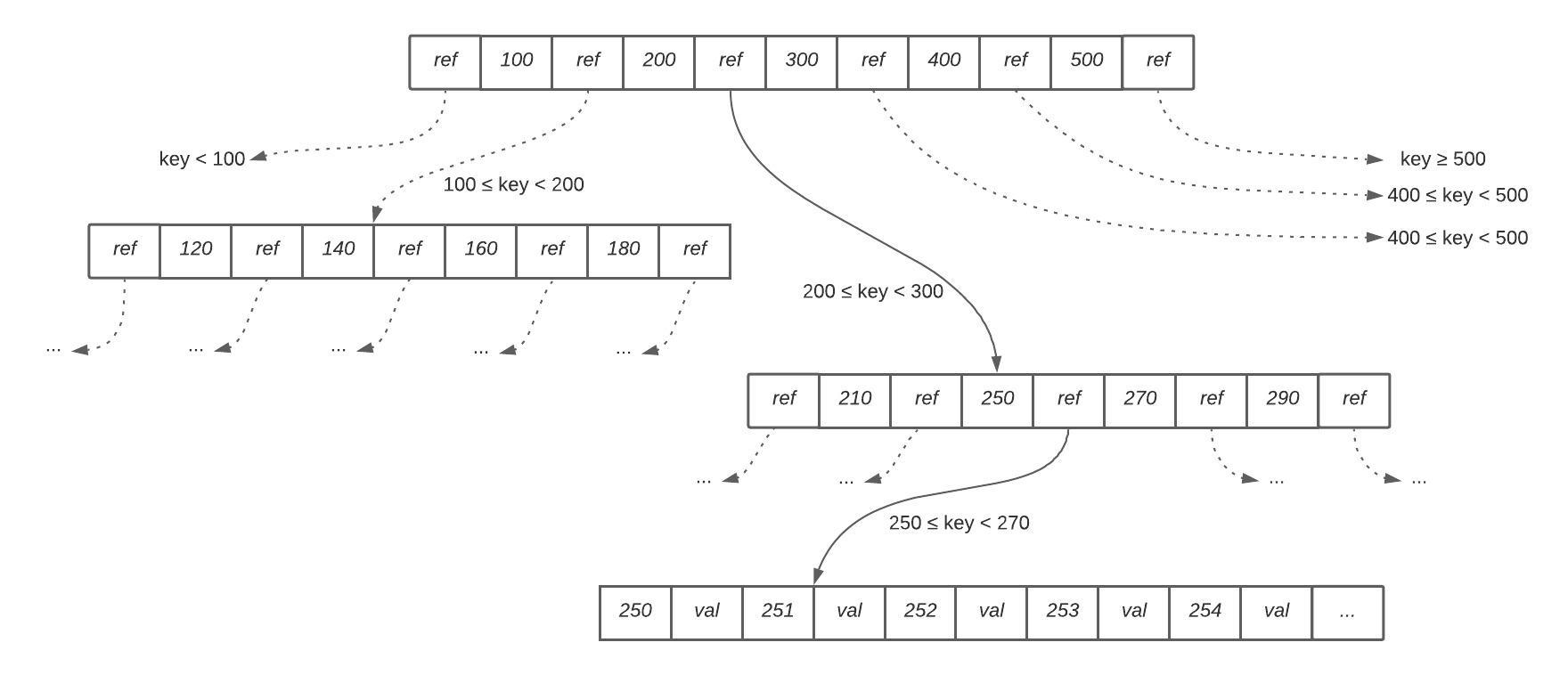
Such a structure allows implementing indexing following a binary search tree principle. One page is designated as a root that contains a number of keys and references to child pages, while child pages are responsible for storing a continuous range of keys and either references or values as shown on Figure 1 below.
CRUD operations
As you can see, in order to find an element we just need to follow a path from the top of the tree to the bottom, up to a page containing an individual key (a leaf page), which gives a very predictable and stable query performance. Additional point in favor of query performance is the fact that the key is stored only in one place, so unlike log-structured indexes, there is no need to check multiple segments to find a value.
Apart from query performance, such index structure allows maintaining similar qualities for updates as well. The only difference between reading and updating the value is the update itself, which is just one extra step.
Please note that actual values can be stored within the index or separately. The latter approach is called a heap file and in this case the index is simply referring to data which is stored separately in an unordered heap file. The alternative approach is called Clustered index and it assumes that values are stored within the index itself. Clustered index is used when the additional leap from the index to a heap file is too much of a performance overhead for reads. In this article I am mostly focusing on Heap page index. Please refer to Clustered index vs. heap if you want to learn more about the differences between two approaches.
However, if the new key needs to be written, then we need to find a page whose range includes the new key and add it there. If there is not enough space in the page to accomodate a new key, then the range needs to be split by two and the parent page - updated.
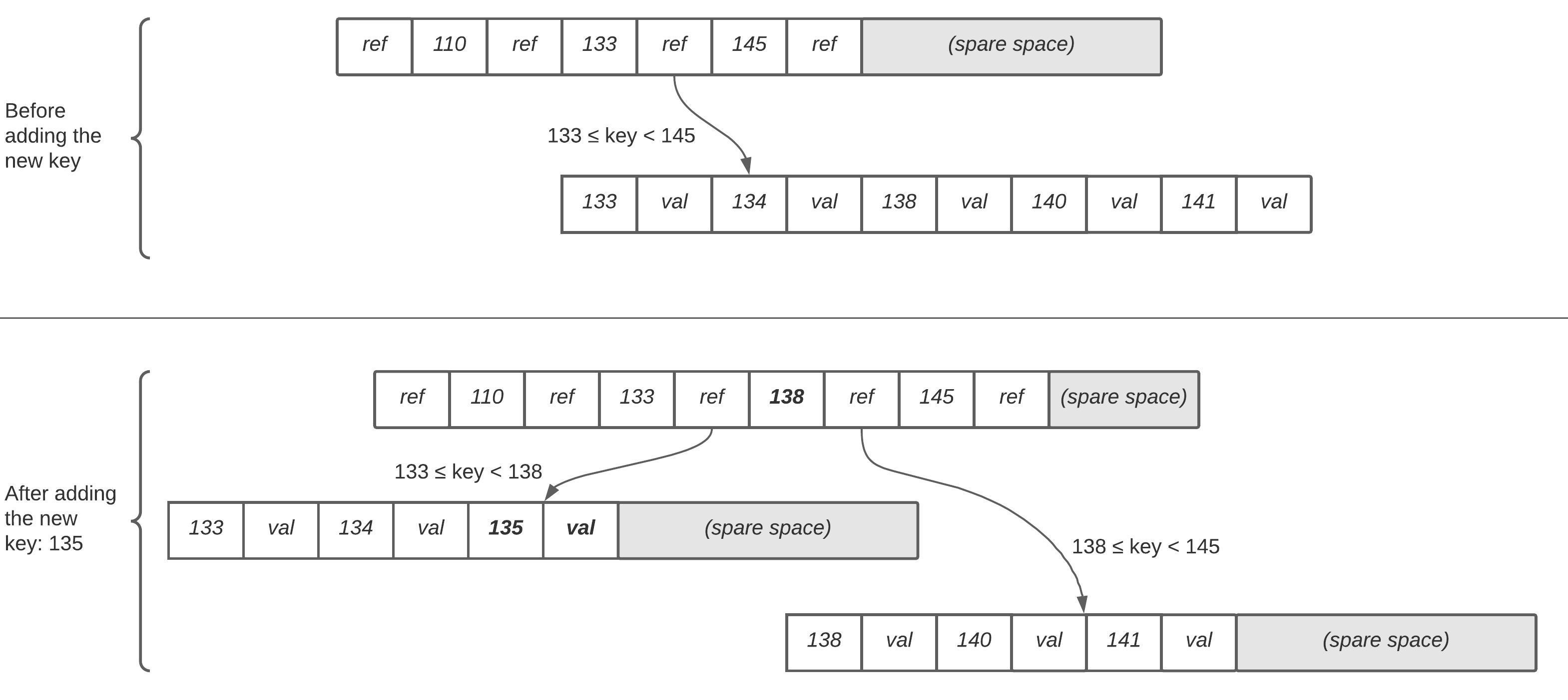
Generally, underlying write operations of a B-tree require to override a whole page on a disk with new data. In case of a page split, the complexity of operation increases even further as instead of overriding just one page, we need to write two new pages that were split as well as overriding the parent one. As a result, LSM-trees are typically considered faster for writes, whereas B-trees - faster for reads.
Even though the writes are typically slower with B-trees, the algorithm described above is very mature and remains one of the most popular on a market. It ensures that the tree remains balanced all the time and a B-tree with n keys always has a depth O(log n). Generally we do not need to make a tree too "deep", for example, a four-level tree with 4 KB pages and 500 references to child pages per page can store up to 256 TB of information.
Number of references to child pages is called Branching factor.
So far we reviewed only read, update and create operations, but there is another one - delete. Deleting the key from a B-tree is a little more tricky as if the tree remains balanced once we remove the key then there is nothing else to do, but if the tree becomes unbalanced, then rebalancing is required. This topic is beyond the scope of the article, but you can read more about it here.
Usage and production implementation
B-trees are traditionally used in relational databases like MySQL, PostgreSQL, etc., however, many non-relational databases use them too.
Production implementations of B-tree indexes may include multiple optimizations like write ahead log, key abbreviation, specific data allocation strategies on a disk, introduction of pointers to sibling pages, implementation of fractal trees, etc., but this is quite complex and may be a good topic for another article.
Conclusion
B-tree index is a very mature and the most commonly used index structure that has its pros and cons. As we found out earlier, they introduce some overhead in case of create and delete operations, but provide plenty of benefits for frequent reads. B-trees do not use a compaction process which saves a lot of disk bandwidth and can be very useful in case of high I/O use cases. They are very ingrained in the architecture of databases and provide consistently good performance for many workloads (60.5% of all DBs are relational as of March, 2019), so they are not going anywhere anytime soon.