During my career I worked with many programming languages, paradigms, design principles, architectures, etc., however, machine learning has always been an unknown and scary territory for me, so a couple of months ago I decided to figure out what this machine learning hype is all about. My good friend and colleague Jonathan Rioux, who is head of Canadian Data Science practice in EPAM Systems, recommended me to start with a free course provided by Fast.ai, and I followed his advice. To be frank, initially I was a bit sceptical about free courses as usually they do not provide much value, but these guys surprised me a lot. This resource provides tons of well structured information and gives an understanding of quite complex topics! When I started writing this article I set myself a goal to explain how machine learning works under the hood, and decided to follow an example established by fast.ai, so I will base my explanation on the problem of handwriting recognition. I have a very deep connection with this problem as it used to be a topic of my PhD research and I dedicated more than a decade of my life to it. But, before we start solving the problem we need to understand why it is that so difficult to recognize handwriting and what tools we can use.
Problem definition
I think the most famous and widely known example is doctor prescriptions, I assume that almost every person at least once struggled to understand what is written on a piece of paper given by a doctor. This example pushes us towards a bit wider issue. We are all different, we have our own characters, habits, behaviour and, moreover, we write differently! So, why is it a problem? Traditional software development is based on predefined rules, so that developers define logic that is based on conditions, operations and loops. Traditional applications usually expect input to be standardized to some extent, so infinite variety of handwriting variations doesn’t really fit to this concept. We simply cannot create a finite number of rules to handle an infinite number of handwritings.
Tools
Historically Data Scientists (megaminds standing behind machine learning invention and creators of whole new buzzword dictionaries) were using Python as one of their main programming languages and Jupyter Notebooks as their development environment. Python itself is an extremely slow programming language, so actual computational logic is usually written on C using CUDA platform and performed on GPU, but we do not need to worry about it as this code has already been implemented in libraries like TensorFlow, PyTorch, etc. Moving forward, we will be using only Python with a couple of additional libraries like PyTorch and fast.ai.
There are a number of services available online that allow you to host your Jupyter Notebooks without a need to install everything locally. I have been using Gradient provided by a GPU-accelerated cloud platform called Paperspace. It is free, but your server can be running for up to 6 hours. There is a good Fast.ai article dedicated to the process of getting started, so I highly recommend you to check it if you want to try all the examples yourself.
Data
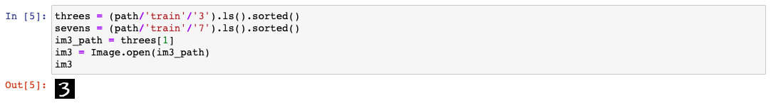
As you could guess, no recognition is possible without the data being recognized. To solve this problem we will be using one of the most famous image databases that contains handwritten digits, namely MNIST Database. It contains 60000 examples of handwritten digits to be used for training purposes, as well as a validation set containing 10000 examples that are used to check how good a trained machine learning model is. Recognizing all the digits is a non-trivial task, so to get a basic understanding about how machine learning works in general we will limit ourselves with two digits, for example, 3 and 7.
Fast.ai provides shortened version of MNIST database that fits to our purpose, to start using it we need to open Jupyter Notebook, install all dependencies (Gradient provides virtual machine with all the dependencies installed) and execute following code:
1 | !pip install -Uqq fastbook |
Jupyter doesn't show if data was correctly downloaded, so we need to check it ourselves by calling ls() function on path variable that represents the path to the folder with data:

Now when the data is prepared we can move forward and start thinking about its recognition.
How computer sees images
In order to start working with images we need to develop a strong understanding of how computers see them. All of our monitors, TVs, phone displays, etc. are using the same technology that is based on pixels, which is a small colored dot. So, in order to display an image the screen needs to represent it as a plane assembled of dots. Computers also need to know what color to display for each pixel, but it doesn’t know what color itself is, so all the colors are represented as a set of numbers, for example, as a combination of [Red, Green, Blue], where intensity of each color varies between 0 and 255. As a result, each image is a matrix of color combinations, like [255,255,255]. For black and white images only one number is used instead of three that represents intensity of color. For example, 0 means that there is no color at all and 255 means that color is black (or vice versa), while everything in between is 253 shades of grey. For example, let’s open one of the images:
1 | threes = (path/'train'/'3').ls().sorted() |
Now we can convert it into an array to check how computer sees it:
1 | array(im3)[0:28,4:25] |
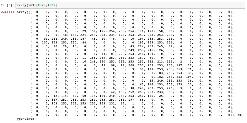
As you can see in computer memory it is a matrix each cell of which is corresponding to a particular pixel with the color code inside.
Author note: Some scientists who work with digital images like with normal once. They approximate each pixel with an integer dot on a Cartesian plane and then perform Cartesian operations, like finding a Cartesian distance between pixels. To me trying to find a Cartesian distance between elements of a matrix sounds a bit silly and, moreover, it results in a significant quality loss.
Basic recognition
Let's think together about how those digits can be recognized? First that comes to my mind is simple comparison where we compare different numbers with ideal (or ethalon) digit and see how similar they are, but we have two problems here:
- We have no idea how ideal 3 or ideal 7 looks like.
- We do not know how to compare them.
We can address them one by one.
Our first model
To solve the first problem, instead of having an ideal digit (which is almost impossible to create) we can use some “mean” (or “average”) digit that will be serving as a model of an ideal digit. Considering that each colored pixel value is actually a number in a range between 0 and 255 it should be possible to create a mean digit by stacking all similar digits together (for example, simply put all threes on top of each other) and calculating a mean color value for each corresponding pixel. In this way we can generate a new digit that assembles qualities of each image that was used to generate it. As a result of this manipulation each pixel of the newly created image will inherit properties of all the pixels it was created from. Therefore, if all of those pixels were black, then the resulting pixel will be black as well, but if some of them were white then the resulting one will be more greyish.
Let's see how it may look like in practice:
1 | stacked_sevens = torch.stack(seven_tensors).float()/255 |
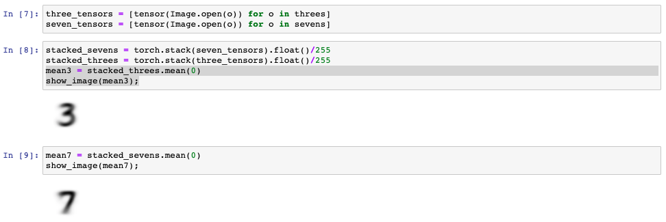
Those are not particularly beautiful, but they represent a "mean digit" and can be used as a model of ethalon digit.
Сomparison
As we have already seen, images represented in computer memory as two dimensional matrices and to be able to compare them we need to make sure that they are of the same size. Fortunately, the Python libraries solve this problem for us by providing multiple image transformation options, but this is far beyond the scope of the current article, so going forward we will assume that images have the same size, colors and other comparable attributes.
Okay, so we have a bunch of different threes, sevens and two averaged digits. In the school course of math we were taught that to check how different two numbers are we need to subtract them and take modulus of the result, i.e. if the result is negative, then we need to make it positive. This simple calculation works with images as well, although we need to do it for every pixel in the image and then take the mean value of all resulting numbers. This approach is called mean absolute difference or L1 norm (I have already warned you about buzzword dictionary).
It is not always convenient to perform such operations on matrices as we need to navigate two directions (horizontally and vertically). To solve this issue, before being compared matrices transformed into vectors by sequentially appending bottom rows to the end of preceding ones, i.e. 10th row will be appended to the end of 9th one, then 9th row will be appended to the end of 8th, etc.
Another approach, instead of taking modulus of difference, assumes taking squares of difference (which makes it positive) and then taking the square root of the result. This approach is called root mean squared error (RMSE) or L2 norm.
To understand if any given digit is three or seven we can simply check if the “distance”, calculated using logic described above, to ideal three is less than to ideal seven and vice versa.
In order to show how it works in practice we need to use the verification set as those threes and sevens did not participate in creating "ideal" digits.
1 | valid_3_tens = torch.stack([tensor(Image.open(o)) |
We will be using mean average function to calculate the difference between digits and is_3 function to check whether digit is three or seven:
1 | def mnist_distance(a,b): return (a-b).abs().mean((-1,-2)) |
We can also calculate how good our initial model performs using accuracy function:
1 | accuracy_3s = is_3(valid_3_tens).float() .mean() |
![]() The numbers above mean that average accuracy of our initial model is 95.11%, which is not bad at all, but we can do better than that.
The numbers above mean that average accuracy of our initial model is 95.11%, which is not bad at all, but we can do better than that.
The problem with the current approach is that it is not exactly machine learning as it cannot learn anything.
Converting model into a machine learning one
To figure out what needs to be done to make our model learn we first need to understand how it works. As you remember, we calculated the mean color value for each pixel of the image, i.e. if our image was 28x28 pixels, then we calculated 784 values. In other words we calculated 784 parameters and then, to calculate the difference between an image and ideal model, we used subtraction between actual value of image pixels and corresponding parameters of the model. Now it’s time to change the approach to make our model learn.
To solve this issue we will be using a similar thinking process, however, for simplicity we will rename our 784 parameters into weights and, instead of calculating mean value of pixels, we will assign them a probability of a pixel being black for a particular digit. As a result, we will be having a matrix defining probability of corresponding pixels to be black (matrix itself will define an overall probability of an image to be three or seven, or whatever else), but how can we use it?
Well, we cannot find distance between an image and probability, but if we look closer it opens another opportunity. For instance, if we multiply the probability of a pixel to be black to its value we can get either a high value if probability is high and actual pixel is black, or much lower value otherwise. So, if we take a weights matrix created for “threes”, calculate the mentioned product for all pixels and sum it up, then we get either a high value if the image is actually three or lower one in the opposite case.
As a result, our new model function will look like following:
1 | def probability_of_three(x,w) = (x*w).sum() |
where x is an actual image (i.e. matrix of color codes) and w is matrix of weights (probabilities).
Traditionally, another parameter is being added the function a bit more flexible, that parameter is called bias, which makes our model looks like a linear function:
1 | def linear(x) = (x*w).sum() + bias |
However, to optimize calculation performance and to perform all multiplications at once, data science engineers use matrix multiplication which allows calculating all x*w products at once (this topic is beyond the scope of current article), so the final model can be optimized even further:
1 | def linear1(x) = x@w + bias |
Combination of weights and bias is called model parameters.
This is all good, but how does this thing learn? Well, it doesn’t yet… However, by changing weights we can either make it better or worse, i.e. we are one step closer to make it learn!
Before we dive deeper into a learning we need to define a way of measuring results, so that we know if learning actually helps making the results better or worse. As it was mentioned earlier there are two ways of measuring results, namely L1 norm and RMSE. We have already used L1 before, so this time we will be using RMSE:
1 | def mse(preds, targets): return ((preds-targets)**2).mean() |
Important to note that the validation set provided by the image database is actually used to measure how good the model is performing. It contains images that we need to use for model validation and expected results. As you can see our
msefunction above (we will call is loss function going forward) uses both values, the ones predicted by model and expected values from the validation set.
If you have seen predictions of machine learning before, it usually has a form of percentage which gives us more or less confidence in results, depending on the value. To achieve the same we need to adjust our loss function a bit more. Taking into account that difference between predictions and targets can be quite substantial we need to standardize the result. Also, we know that values in percent are usually between 0 and 1, where 1 corresponds to 100%. There is a mathematical function that might be handy in this situation which called sigmoid, the plot of this function looks like following:
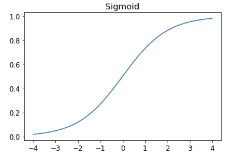
As you can see from the graphic, this function produces results between 0 and 1 for any parameter, which is exactly what we need. So, let's rewrite our loss function one more time (we will also rename it to mnist_loss):
1 | def mnist_loss(preds, targets): |
torch.where function is used to choose what value to return. If the expected value from the validation set is 1, then it returns 1-preds, otherwise preds. Please note that by taking sigmoid of predictions we make it be in a range between 0 and 1, so if we model prediction matches expected one with 100% confidence 0 loss will be returned.
Now, when we know how to measure results, we can get back to the learning process. If we look at our linear1 from a little bit different angle, then we can see that it is a simple mathematical function, like the ones we have seen during our school curriculum:
1 | y = f(x) |
where y is a result of our function and f(x) in our case equals to x@w + bias. Therefore, learning would actually mean an optimization of weights and bias in a way that loss calculated based on the function's result (i.e. y) becomes smaller.
We may also remember from school curriculum that there is a way to understand how function results change in case of parameters change, and this way is called derivative! The derivative of a function is another function, which calculates the change rather than value.
Fast.ai: For instance, the derivative of the quadratic function at the value 3 tells us how rapidly the function changes at the value 3.
As I mentioned before, Data Scientists are quite innovative dudes and dudettes, so even though we have derivative function in place, they came up with another fancy term that means almost the same, namely gradient. Gradient measures for each weight how changing its value would change the loss. Also, iterative application of gradient function to change parameters called Stochastic Gradient Descent or simply SGD.
So, to update our parameters (i.e. weights and bias), we need to apply model function, calculate loss, then calculate gradient (read is as derivative) for each of weights and subtract gradient value multiplied by learning rate from the initial weight value. Learning rate is usually a pretty small number (like 0.00001 or 1E-5) that is used to reduce the speed of weights change. It is an empirically calculated value, which means there is no exact formula for it. So, here is the formula for weights update:
1 | w -= gradient(w) * lr |
where lr is the learning rate. By the way, bias value is being updated in the same way.
Interestingly, but we do not need to calculate initial values of weights and bias as they will be changed anyways, therefore their initial values can be chosen randomly.
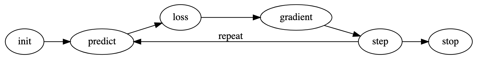
Now, when we know all the important information, let's bring it all together. So, to build a machine learning system from scratch we need:
- Pick or create a model that works best for the task (we reviewed only a trivial linear model, but there are much more than that).
- Randomly initialize model parameters (i.e. weights and bias(es)).
- Predict results using the model on a training set (i.e. calculate function results for each image).
- Calculate loss.
- Calculate gradient.
- Adjust parameters based on gradient.
- Repeat process starting from step #3 until accuracy satisfies the needs.
- Stop once we achieved desired accuracy.
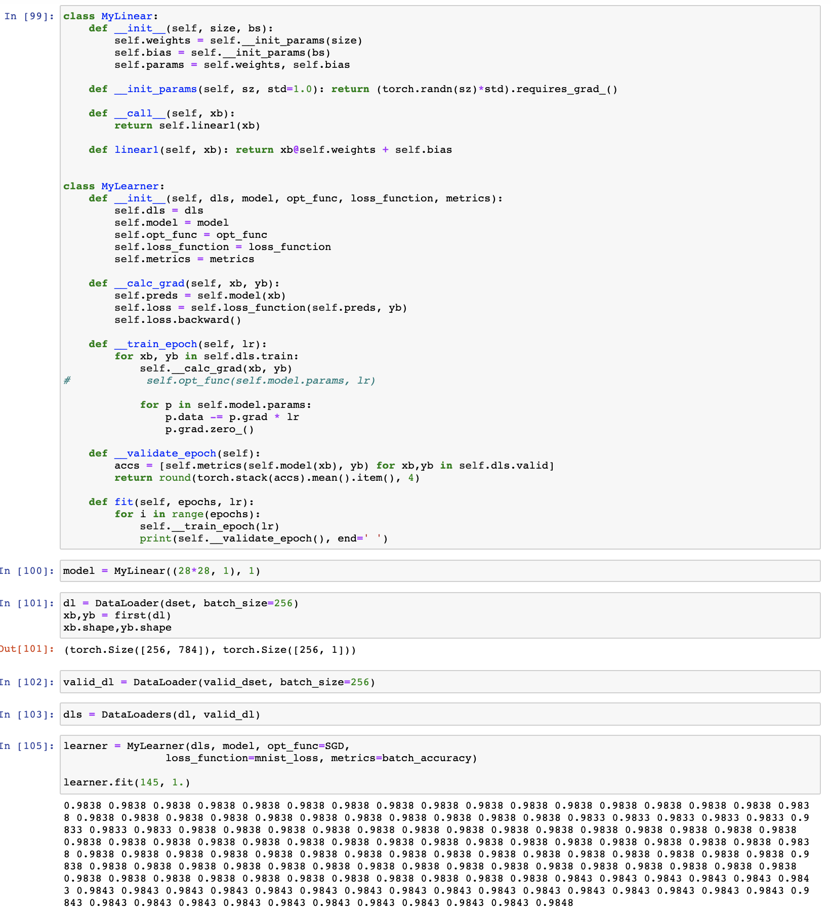
Using my very simplistic custom implementation of the logic above and after a lot of training I was able to achieve 98.48% of accuracy, which is not bad, but also not a limit.
To improve our result we can add more layers to the model, i.e. using not one model function, but a couple of them sequentially, so output of one function becomes an input for the next one, like y(g(f(x))). Models like these are called neural nets and starting from this moment simple machine learning transforms into a fancy deep learning! Deep learning simply means that the model has more than one layer. Here is an example of such model:
1 | def simple_net(xb): |
Note, that each of linear functions has its own set of weights as well as its own bias.
With this model I was able to achieve 98.528% of accuracy, which is a bit better than it used to be, however, it also required a lot of training. But can it be better? Yes. To make the result even better we can use one of the existing pretrained models with a lot more layers, for instance resnet18, where 18 is the number of layers.
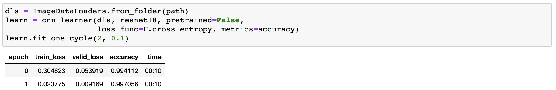
This model gives us 99.7% of accuracy with only 2 iterations of training (by the way, they are called epochs), which is almost 100% of accuracy! After achieving this great result I considered myself the greatest data scientist in the world and decided to retire... But then I realized that I have a couple more things to learn, so I will continue sharing my findings related to different areas of technologies in the following posts.
PS: You can find my Jupyter Notebook here: GitHub.
Conclusion
Now you know that the concept of machine learning is not complex by itself. We started with simple image comparison and slowly evolved our algorithms to a state of art deep learning machine in a very limited time. As I mentioned before, machine learning has always been something like a black magic to me, but after a couple of hours spent with it I understood that it is a simple mathematical concept by its nature. I remember learning Rosenblatt perceptron in the third year of university, but at that time my attention was mostly focused on my parties, friends and opposite sex, so I did not have time for such “unnecessary things” as machine learning. Of course, there is much more in ML than that, but now we have a foundation, which can serve as a basis for future research. I wish you luck and hope it was useful.